
Preparing a state with antiferromagnetic order in the Ising model
This notebook illustrates how to use Pulser to build a sequence for studying an antiferromagnetic state in an Ising-like model. It is based on 10.1103/PhysRevX.8.021070 (external), where arrays of Rydberg atoms were programmed and whose correlations were studied.
We begin by importing some basic modules:
import numpy as npimport matplotlib.pyplot as pltimport qutip
from pulser import Pulse, Sequence, Registerfrom pulser_simulation import QutipEmulatorfrom pulser.waveforms import RampWaveformfrom pulser.devices import AnalogDevice
Waveforms
Section titled “Waveforms”We are realizing the following program

The pulse and the register are defined by the following parameters:
# Parameters in rad/µs and nsOmega_max = 2.0 * 2 * np.piU = Omega_max / 2.0
delta_0 = -6 * Udelta_f = 2 * U
t_rise = 252t_fall = 500t_sweep = (delta_f - delta_0) / (2 * np.pi * 10) * 1000
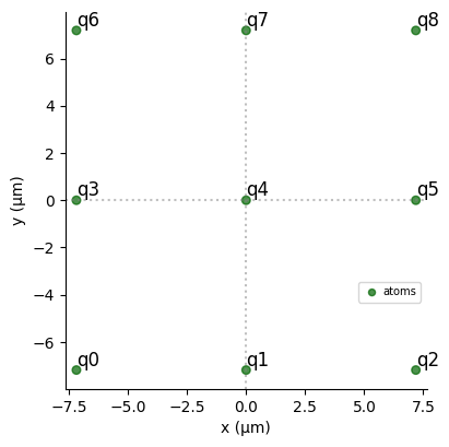
R_interatomic = AnalogDevice.rydberg_blockade_radius(U)
N_side = 3reg = Register.square(N_side, R_interatomic, prefix="q")print(f"Interatomic Radius is: {R_interatomic}µm.")reg.draw()
Interatomic Radius is: 7.186760677748386µm.
Creating my sequence
Section titled “Creating my sequence”We compose our pulse with the following objects from Pulser:
rise = Pulse.ConstantDetuning( RampWaveform(t_rise, 0.0, Omega_max), delta_0, 0.0)sweep = Pulse.ConstantAmplitude( Omega_max, RampWaveform(t_sweep, delta_0, delta_f), 0.0)fall = Pulse.ConstantDetuning( RampWaveform(t_fall, Omega_max, 0.0), delta_f, 0.0)seq = Sequence(reg, AnalogDevice)seq.declare_channel("ising", "rydberg_global")
seq.add(rise, "ising")seq.add(sweep, "ising")seq.add(fall, "ising")
seq.draw()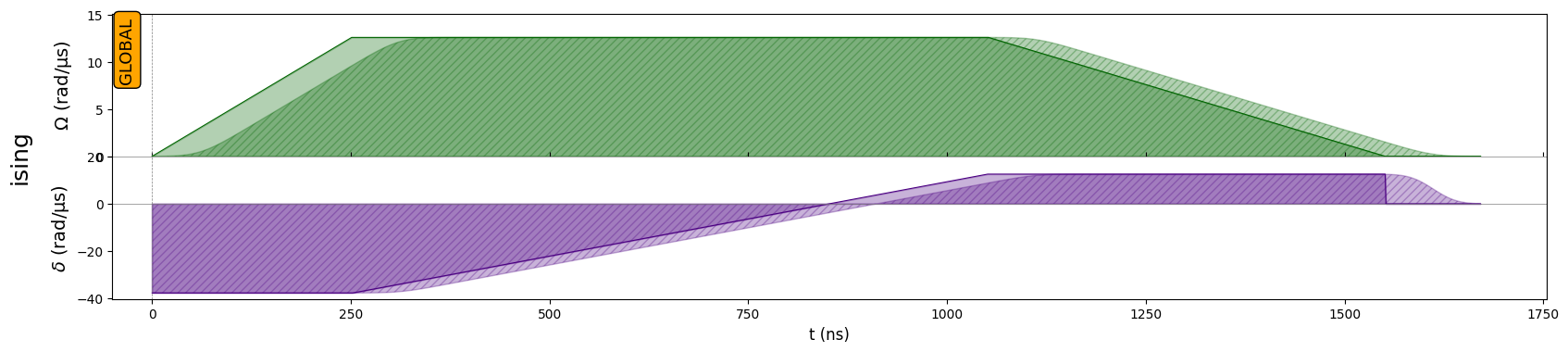
Phase Diagram
Section titled “Phase Diagram”The pulse sequence travels though the following path in the phase diagram of the system (the shaded area represents the antiferromagnetic phase):
delta = []omega = []for x in seq._schedule["ising"]:    if isinstance(x.type, Pulse):        omega += list(x.type.amplitude.samples / U)        delta += list(x.type.detuning.samples / U)
fig, ax = plt.subplots()ax.grid(True, which="both")
ax.set_ylabel(r"$\hbar\delta(t)/U$", fontsize=16)ax.set_xlabel(r"$\hbar\Omega(t)/U$", fontsize=16)ax.set_xlim(0, 3)ax.axhline(y=0, color="k")ax.axvline(x=0, color="k")
y = np.arange(0.0, 6, 0.01)x = 1.522 * (1 - 0.25 * (y - 2) ** 2)ax.fill_between(x, y, alpha=0.4)
ax.plot(omega, delta, "red", lw=2)plt.show()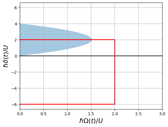
Simulation: Spin-Spin Correlation Function
Section titled “Simulation: Spin-Spin Correlation Function”We shall now evaluate the quality of the obtained state by calculating the spin-spin correlation function, defined as:
where the indicates that we are calculating the connected part, and where the sum is over all pairs whose distance is in the atomic array coordinate (both and are positive or negative integers within the size of the array).
We run a simulation of the sequence:
simul = QutipEmulator.from_sequence(seq, sampling_rate=0.02)results = simul.run(progress_bar=True)
12.9%. Run time:   0.01s. Est. time left: 00:00:00:00
22.6%. Run time:   0.02s. Est. time left: 00:00:00:00
32.3%. Run time:   0.02s. Est. time left: 00:00:00:00
41.9%. Run time:   0.03s. Est. time left: 00:00:00:00
51.6%. Run time:   0.04s. Est. time left: 00:00:00:00
61.3%. Run time:   0.05s. Est. time left: 00:00:00:00
71.0%. Run time:   0.06s. Est. time left: 00:00:00:00
80.6%. Run time:   0.07s. Est. time left: 00:00:00:00
90.3%. Run time:   0.07s. Est. time left: 00:00:00:00
Total run time:   0.08s
Sample from final state using sample_final_state() method:
count = results.sample_final_state()
most_freq = {k: v for k, v in count.items() if v > 10}plt.bar(list(most_freq.keys()), list(most_freq.values()))plt.xticks(rotation="vertical")plt.show()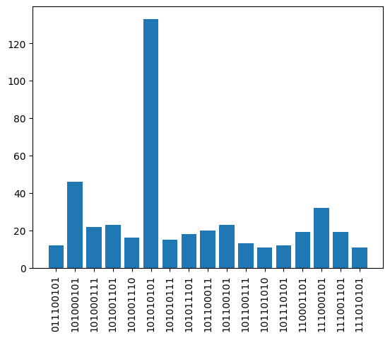
The observable to measure will be the occupation operator on each site of the register, where the Rydberg state represents the excited state.
def occupation(j, N): up = qutip.basis(2, 0) prod = [qutip.qeye(2) for _ in range(N)] prod[j] = up * up.dag() return qutip.tensor(prod)occup_list = [occupation(j, N_side * N_side) for j in range(N_side * N_side)]We define a function that returns all couples for a given :
def get_corr_pairs(k, l, register, R_interatomic): corr_pairs = [] for i, qi in enumerate(register.qubits): for j, qj in enumerate(register.qubits): r_ij = register.qubits[qi] - register.qubits[qj] distance = np.linalg.norm(r_ij - R_interatomic * np.array([k, l])) if distance < 1: corr_pairs.append([i, j]) return corr_pairsThe correlation function is calculated with the following routines:
def get_corr_function(k, l, reg, R_interatomic, state):    N_qubits = len(reg.qubits)    corr_pairs = get_corr_pairs(k, l, reg, R_interatomic)
    operators = [occupation(j, N_qubits) for j in range(N_qubits)]    covariance = 0    for qi, qj in corr_pairs:        covariance += qutip.expect(operators[qi] * operators[qj], state)        covariance -= qutip.expect(operators[qi], state) * qutip.expect(            operators[qj], state        )    return covariance / len(corr_pairs)

def get_full_corr_function(reg, state):    N_qubits = len(reg.qubits)
    correlation_function = {}    N_side = int(np.sqrt(N_qubits))    for k in range(-N_side + 1, N_side):        for l in range(-N_side + 1, N_side):            correlation_function[(k, l)] = get_corr_function(                k, l, reg, R_interatomic, state            )    return correlation_function
With these functions, we operate on the final state of evolution obtained by our simulation.
final = results.states[-1]correlation_function = get_full_corr_function(reg, final)expected_corr_function = {}xi = 1 # Estimated Correlation Lengthfor k in range(-N_side + 1, N_side): for l in range(-N_side + 1, N_side): kk = np.abs(k) ll = np.abs(l) expected_corr_function[(k, l)] = (-1) ** (kk + ll) * np.exp( -np.sqrt(k**2 + l**2) / xi )A = 4 * np.reshape( list(correlation_function.values()), (2 * N_side - 1, 2 * N_side - 1))A = A / np.max(A)B = np.reshape( list(expected_corr_function.values()), (2 * N_side - 1, 2 * N_side - 1))B = B * np.max(A)
for i, M in enumerate([A.copy(), B.copy()]): M[N_side - 1, N_side - 1] = None plt.figure(figsize=(3.5, 3.5)) plt.imshow(M, cmap="coolwarm", vmin=-0.6, vmax=0.6) plt.xticks(range(len(M)), [f"{x}" for x in range(-N_side + 1, N_side)]) plt.xlabel(r"$\mathscr{k}$", fontsize=22) plt.yticks(range(len(M)), [f"{-y}" for y in range(-N_side + 1, N_side)]) plt.ylabel(r"$\mathscr{l}$", rotation=0, fontsize=22, labelpad=10) plt.colorbar(fraction=0.047, pad=0.02) if i == 0: plt.title( r"$4\times\.g^{(2)}(\mathscr{k},\mathscr{l})$ after simulation", fontsize=14, ) if i == 1: plt.title( r"Exponential $g^{(2)}(\mathscr{k},\mathscr{l})$ expected", fontsize=14, ) plt.show()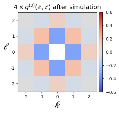
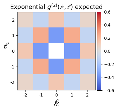
Note that the correlation function would follow an exponential decay (modulo finite-size effects), which is best observed at larger system sizes (see for example https://arxiv.org/pdf/2012.12268.pdf (external))
np.around(A, 4)
array([[-0.0039, -0.0385,  0.0866, -0.0385, -0.0039],
       [-0.0385,  0.1654, -0.345 ,  0.1654, -0.0385],
       [ 0.0866, -0.345 ,  1.    , -0.345 ,  0.0866],
       [-0.0385,  0.1654, -0.345 ,  0.1654, -0.0385],
       [-0.0039, -0.0385,  0.0866, -0.0385, -0.0039]])
np.around(B, 4)
array([[ 0.0591, -0.1069,  0.1353, -0.1069,  0.0591],
       [-0.1069,  0.2431, -0.3679,  0.2431, -0.1069],
       [ 0.1353, -0.3679,  1.    , -0.3679,  0.1353],
       [-0.1069,  0.2431, -0.3679,  0.2431, -0.1069],
       [ 0.0591, -0.1069,  0.1353, -0.1069,  0.0591]])
Néel Structure Factor
Section titled “Néel Structure Factor”One way to explore the line on the phase diagram is to calculate the Néel Structure Factor, , which should be highest when the state is more antiferromagnetic. We will sweep over different values of to show that the region is indeed where the antiferromagnetic phase takes place.
def get_neel_structure_factor(reg, R_interatomic, state):    N_qubits = len(reg.qubits)    N_side = int(np.sqrt(N_qubits))
    st_fac = 0    for k in range(-N_side + 1, N_side):        for l in range(-N_side + 1, N_side):            kk = np.abs(k)            ll = np.abs(l)            if not (k == 0 and l == 0):                st_fac += (                    4                    * (-1) ** (kk + ll)                    * get_corr_function(k, l, reg, R_interatomic, state)                )    return st_fac
def calculate_neel(det, N, Omega_max=2.0 * 2 * np.pi): # Setup: U = Omega_max / 2.0 delta_0 = -6 * U delta_f = det * U
t_rise = 252 t_fall = 500 t_sweep = int((delta_f - delta_0) / (2 * np.pi * 10) * 1000) t_sweep += ( 4 - t_sweep % 4 ) # To be a multiple of the clock period of AnalogDevice (4ns)
R_interatomic = AnalogDevice.rydberg_blockade_radius(U) reg = Register.rectangle(N, N, R_interatomic)
# Pulse Sequence rise = Pulse.ConstantDetuning( RampWaveform(t_rise, 0.0, Omega_max), delta_0, 0.0 ) sweep = Pulse.ConstantAmplitude( Omega_max, RampWaveform(t_sweep, delta_0, delta_f), 0.0 ) fall = Pulse.ConstantDetuning( RampWaveform(t_fall, Omega_max, 0.0), delta_f, 0.0 )
seq = Sequence(reg, AnalogDevice) seq.declare_channel("ising", "rydberg_global") seq.add(rise, "ising") seq.add(sweep, "ising") seq.add(fall, "ising")
simul = QutipEmulator.from_sequence(seq, sampling_rate=0.2) results = simul.run()
final = results.states[-1] return get_neel_structure_factor(reg, R_interatomic, final)N_side = 3occup_list = [occupation(j, N_side * N_side) for j in range(N_side * N_side)]
detunings = np.linspace(-1, 5, 20)results = []for det in detunings: print(f"Detuning = {np.round(det,3)} x 2π Mhz.") results.append(calculate_neel(det, N_side))plt.xlabel(r"$\hbar\delta_{final}/U$")plt.ylabel(r"Néel Structure Factor $S_{Neel}$")plt.plot(detunings, results, "o", ls="solid")plt.show()max_index = results.index(max(results))print( f"Max S_Neel {np.round(max(results),2)} at detuning = {np.round(detunings[max_index],2)} x 2π Mhz.")
Detuning = -1.0 x 2π Mhz.
Detuning = -0.684 x 2π Mhz.
Detuning = -0.368 x 2π Mhz.
Detuning = -0.053 x 2π Mhz.
Detuning = 0.263 x 2π Mhz.
Detuning = 0.579 x 2π Mhz.
Detuning = 0.895 x 2π Mhz.
Detuning = 1.211 x 2π Mhz.
Detuning = 1.526 x 2π Mhz.
Detuning = 1.842 x 2π Mhz.
Detuning = 2.158 x 2π Mhz.
Detuning = 2.474 x 2π Mhz.
Detuning = 2.789 x 2π Mhz.
Detuning = 3.105 x 2π Mhz.
Detuning = 3.421 x 2π Mhz.
Detuning = 3.737 x 2π Mhz.
Detuning = 4.053 x 2π Mhz.
Detuning = 4.368 x 2π Mhz.
Detuning = 4.684 x 2π Mhz.
Detuning = 5.0 x 2π Mhz.
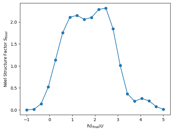
Max S_Neel 2.32 at detuning = 2.47 x 2π Mhz.