
XY Spin Chain
We introduce here a new mode of interaction between the atoms driven by the dipole-dipole interaction. This mode is called the XY mode. The interaction hamiltonian of a system of qubits is now given by
where , is the distance between atom and atom , and is a coefficient dependent on the device and taken as for the MockDevice.
The final hamiltonian of the system is
The Rydberg states involved are different from the ones of the Ising interaction, they are and .
More details on the XY mode can be found in the following reference: Barredo et al. 2014 (external)
import numpy as npimport matplotlib.pyplot as pltimport qutip
import pulserfrom pulser import Pulse, Sequence, Registerfrom pulser_simulation import QutipEmulatorfrom pulser.devices import MockDevicefrom pulser.waveforms import BlackmanWaveform
Rabi oscillations of 1 atom
Section titled “Rabi oscillations of 1 atom”We start by showing Rabi oscillation in the XY mode in the case of a unique atom as shown in the figure 1 (c) of the reference (external). In a similar way as the Ising mode, the atom will oscillate between the two energy levels. The XY mode is only available in the mw_global channel. We initialize the register and instantiate the channel.
coords = np.array([[0, 0]])qubits = dict(enumerate(coords))
reg = Register(qubits)seq = Sequence(reg, MockDevice)seq.declare_channel("MW", "mw_global")
We then add a simple constant rabi pulse of amplitude MHz and run the simulation. The measurement is necessarily done in the XY basis.
simple_pulse = Pulse.ConstantPulse(4000, 2 * np.pi * 4.6, 0, 0)seq.add(simple_pulse, "MW")seq.measure(basis="XY")
sim = QutipEmulator.from_sequence(seq)
results = sim.run(progress_bar=True, nsteps=5000)
10.0%. Run time:   0.02s. Est. time left: 00:00:00:00
20.0%. Run time:   0.05s. Est. time left: 00:00:00:00
30.0%. Run time:   0.07s. Est. time left: 00:00:00:00
40.0%. Run time:   0.10s. Est. time left: 00:00:00:00
50.0%. Run time:   0.12s. Est. time left: 00:00:00:00
60.0%. Run time:   0.15s. Est. time left: 00:00:00:00
70.0%. Run time:   0.17s. Est. time left: 00:00:00:00
80.0%. Run time:   0.19s. Est. time left: 00:00:00:00
90.0%. Run time:   0.22s. Est. time left: 00:00:00:00
Total run time:   0.24s
We plot the expectation of the excitation of the atom over the time.
def excitation(j, total_sites):    """The |1><1| projector operator on site j."""    prod = [qutip.qeye(2) for _ in range(total_sites)]    prod[j] = (qutip.qeye(2) - qutip.sigmaz()) / 2    return qutip.tensor(prod)

excited = excitation(0, 1)plt.figure(figsize=[16, 6])results.plot(excited)plt.xlabel("Pulse duration (ns)", fontsize="x-large")plt.ylabel("Excitation of the atom", fontsize="x-large")plt.show()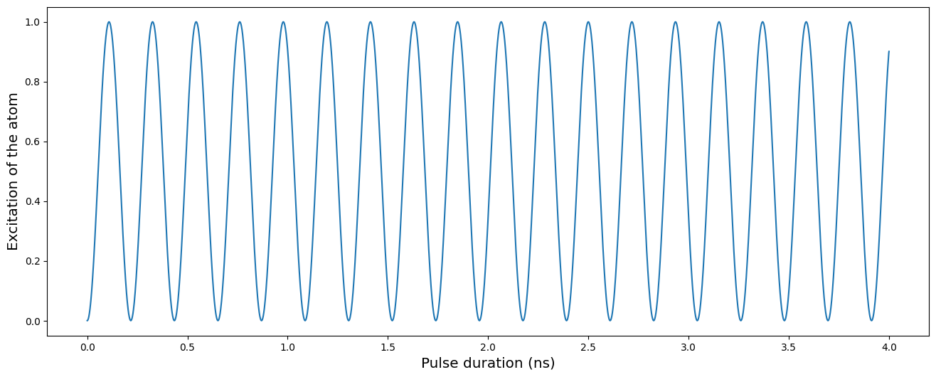
Spin chain of 3 atoms
Section titled “Spin chain of 3 atoms”We now simulate the free evolution of a spin chain of 3 atoms, starting with 1 excitation in the initial state as shown in the figure 3 (c) of the reference (external).
coords = np.array([[-8.0, 0], [0, 0], [8.0, 0]])qubits = dict(enumerate(coords))
reg = Register(qubits)seq = Sequence(reg, MockDevice)seq.declare_channel("ch0", "mw_global")reg.draw()
# State preparation using SLM maskmasked_qubits = [1, 2]seq.config_slm_mask(masked_qubits)masked_pulse = Pulse.ConstantDetuning(BlackmanWaveform(200, np.pi), 0, 0)seq.add(masked_pulse, "ch0")
# Simulation pulsesimple_pulse = Pulse.ConstantPulse(7000, 0, 0, 0)seq.add(simple_pulse, "ch0")seq.measure(basis="XY")
sim = QutipEmulator.from_sequence(seq, sampling_rate=1)results = sim.run(nsteps=5000)
excited_list = [excitation(j, 3) for j in range(3)]
expectations = results.expect(excited_list)
plt.figure(figsize=[16, 18])plt.subplot(311)plt.plot(expectations[0])plt.ylabel("Excitation of atom 0", fontsize="x-large")plt.xlabel("Time (ns)", fontsize="x-large")plt.subplot(312)plt.plot(expectations[1])plt.ylabel("Excitation of atom 1", fontsize="x-large")plt.xlabel("Time (ns)", fontsize="x-large")plt.ylim([0, 1])plt.subplot(313)plt.plot(expectations[2])plt.ylabel("Excitation of atom 2", fontsize="x-large")plt.xlabel("Time (ns)", fontsize="x-large")plt.show()
External field and angular dependency
Section titled “External field and angular dependency”An external magnetic field can be added to the experiment, and will modify the hamiltonian. The XY Hamiltonian is then
where is the angle between the vector of the two atoms and the external field as shown on the figure below.

We add an external field along the Y axis, and we put the qubit 2 at the angle such that , and the interaction between the qubits 1 and 2 cancels out. This is done by the method set_magnetic_fieldfrom the Sequence.
This is the principle that enables to create topological phases (external) on long chain of atoms.
coords = np.array([[-1.0, 0], [0, 0], [np.sqrt(2 / 3), np.sqrt(1 / 3)]]) * 8.0qubits = dict(enumerate(coords))
reg = Register(qubits)seq = Sequence(reg, MockDevice)seq.declare_channel("ch0", "mw_global")seq.set_magnetic_field(0.0, 1.0, 0)reg.draw()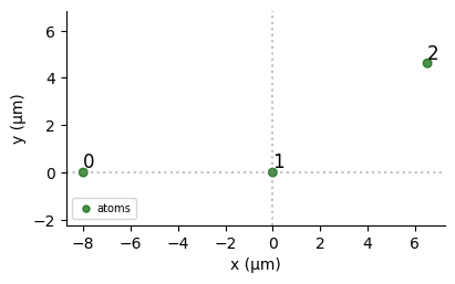
We then simulate again the free evolution from the initial state .
# State preparation using SLM maskmasked_qubits = [1, 2]seq.config_slm_mask(masked_qubits)masked_pulse = Pulse.ConstantDetuning(BlackmanWaveform(200, np.pi), 0, 0)seq.add(masked_pulse, "ch0")
# Simulation pulsesimple_pulse = Pulse.ConstantPulse(7000, 0, 0, 0)seq.add(simple_pulse, "ch0")seq.measure(basis="XY")
sim = QutipEmulator.from_sequence(seq, sampling_rate=1)results = sim.run(progress_bar=True, nsteps=5000)
10.0%. Run time:   0.04s. Est. time left: 00:00:00:00
20.0%. Run time:   0.09s. Est. time left: 00:00:00:00
30.0%. Run time:   0.13s. Est. time left: 00:00:00:00
40.0%. Run time:   0.17s. Est. time left: 00:00:00:00
50.0%. Run time:   0.22s. Est. time left: 00:00:00:00
60.0%. Run time:   0.27s. Est. time left: 00:00:00:00
70.0%. Run time:   0.32s. Est. time left: 00:00:00:00
80.0%. Run time:   0.36s. Est. time left: 00:00:00:00
90.0%. Run time:   0.42s. Est. time left: 00:00:00:00
Total run time:   0.47s
excited_list = [excitation(j, 3) for j in range(3)]
expectations = results.expect(excited_list)
plt.figure(figsize=[16, 18])plt.subplot(311)plt.plot(expectations[0])plt.ylabel("Excitation of atom 0", fontsize="x-large")plt.xlabel("Time ($\mu$s)", fontsize="x-large")plt.ylim([0, 1])plt.subplot(312)plt.plot(expectations[1])plt.ylabel("Excitation of atom 1", fontsize="x-large")plt.xlabel("Time ($\mu$s)", fontsize="x-large")plt.ylim([0, 1])plt.subplot(313)plt.plot(expectations[2])plt.ylabel("Excitation of atom 2", fontsize="x-large")plt.xlabel("Time ($\mu$s)", fontsize="x-large")plt.ylim([0, 1])plt.show()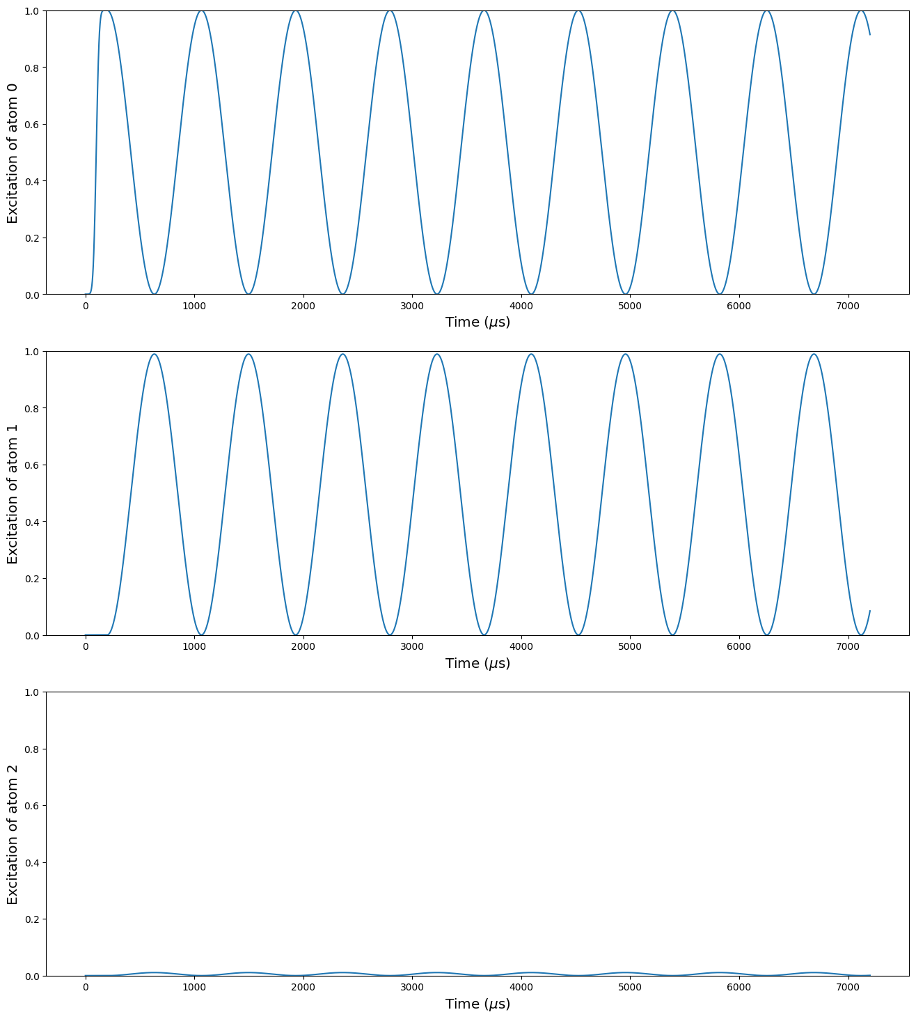
We can see there that there is almost no excitation in the qubit 2. It still remains some because the interaction between the qubits 0 and 2 is not completely negligible.