Creating Size-Dependent States and Operators

The State and Operator classes let you build arbitrary state and operator objects from scratch using the from_state_amplitudes() and from_operator_repr() methods (as shown in Execution on an Emulator and Results and Observables). Also, Operator.from_pauli_string() provides a shortcut for creating Pauli string operators. Together, these objects are used to create initial states, calculate observables such as Fidelity, and find expectation values of custom operators at any desired moment of your Pulser sequence.

A common use case for these is many-body physics simulations, where you often want to:

prepare reference initial states that are non-trivial,
scale the number of qubits to look for trends that persist (or not).

This page presents some simple recipes for defining commonly used states and operators with a variable system size, and how to calculate their expectation values.

Size-dependent Pauli-string operators

Many observables of interest are Pauli-string operators, i.e. tensor products of Pauli matrices acting on different qubits, such as $Z_0 X_1 Z_3$ . These can be built for any system size with Operator.from_pauli_string(), which takes:

eigenstates: the basis the Pauli matrices are defined in,
n_qudits: the number of qubits in the system,
paulis: a mapping between the index of a qubit in the register and the Pauli matrix ("X", "Y" or "Z") applied to it. All the other qubits are applied the identity.

With eigenstates = ("r", "g") (the ground-rydberg basis), Pauli-string operators can be built as follows:

from pulser_simulation import QutipConfig

eigenstates = ("r", "g")

# The operator class comes from the backend's configuration
operator_class = QutipConfig.operator_type

# Z_0 X_1 Z_3 on a system of four qubits
z0x1z3 = operator_class.from_pauli_string(
    eigenstates=eigenstates, n_qudits=4, paulis={0: "Z", 1: "X", 3: "Z"}
)
# The qutip.Qobj associated with this operator
z0x1z3.to_qobj()

Quantum object: dims=[[2, 2, 2, 2], [2, 2, 2, 2]], shape=(16, 16), type='oper', dtype=CSR, isherm=True$$\left(\begin{array}{cc}0 & 0 & 0 & 0 & 1 & \cdots & 0 & 0 & 0 & 0 & 0\\0 & 0 & 0 & 0 & 0 & \cdots & 0 & 0 & 0 & 0 & 0\\0 & 0 & 0 & 0 & 0 & \cdots & 0 & 0 & 0 & 0 & 0\\0 & 0 & 0 & 0 & 0 & \cdots & 0 & 0 & 0 & 0 & 0\\1 & 0 & 0 & 0 & 0 & \cdots & 0 & 0 & 0 & 0 & 0\\\vdots & \vdots & \vdots & \vdots & \vdots & \ddots & \vdots & \vdots & \vdots & \vdots & \vdots\\0 & 0 & 0 & 0 & 0 & \cdots & 0 & 0 & 0 & 0 & 1\\0 & 0 & 0 & 0 & 0 & \cdots & 0 & 0 & 0 & 0 & 0\\0 & 0 & 0 & 0 & 0 & \cdots & 0 & 0 & 0 & 0 & 0\\0 & 0 & 0 & 0 & 0 & \cdots & 0 & 0 & 0 & 0 & 0\\0 & 0 & 0 & 0 & 0 & \cdots & 1 & 0 & 0 & 0 & 0\end{array}\right)$$

Since from_pauli_string() relies on from_operator_repr() under the hood, the resulting operator works with any backend, including remote ones. Any other Operator subclass (e.g. OperatorRepr) can be used in place of QutipConfig.operator_type.

It is straightforward to define families of operators whose support depends on the number of qubits. For instance, the end-to-end correlator $Z_0 Z_{n-1}$ and the parity operator $X^{\otimes n}$ :

from pulser.backend import Operator


def end_to_end_zz(n_qubits: int) -> Operator:
    """Builds Z_0 Z_{n-1} on a system of n_qubits."""
    return operator_class.from_pauli_string(
        eigenstates=eigenstates,
        n_qudits=n_qubits,
        paulis={0: "Z", n_qubits - 1: "Z"},
    )


def x_parity(n_qubits: int) -> Operator:
    """Builds X_0 X_1 ... X_{n-1} on a system of n_qubits."""
    return operator_class.from_pauli_string(
        eigenstates=eigenstates,
        n_qudits=n_qubits,
        paulis={i: "X" for i in range(n_qubits)},
    )

Building reference states

In the same spirit, get_state() builds reference states of arbitrary size via from_state_amplitudes(), which takes a mapping between basis state combinations and their complex amplitudes.

from typing import Type

import numpy as np

from pulser.backend import State, StateRepr


def get_state(
    n_qubits: int,
    state_class: Type[State] = StateRepr,
    state_name: str = "plus",
) -> State:
    """Builds a reference state of size n_qubits.

    Args:
        n_qubits: The number of qubits in the state.
        state_class: The ``State`` subclass to instantiate, usually taken
            from a backend's ``config_type.state_type``.
        state_name: The reference state to build, either "plus" (the
            uniform superposition of all basis states) or "ghz".

    Returns:
        The requested reference state, normalized to 1.

    Raises:
        NotImplementedError: If ``state_name`` is not a known reference
            state.

    Examples:
        >>> # builds (|rrrr> + |gggg>) / sqrt(2)
        >>> get_state(n_qubits=4, state_name="ghz")
    """
    if state_name == "plus":
        # |+>^n_qubits: all 2^n_qubits basis states with equal amplitude
        dim = 2**n_qubits
        amplitudes = {
            # format(i, "0{n}b") writes the integer i as a binary string
            # of fixed length n_qubits, whose digits then index into
            # 'eigenstates' to name the basis state combination
            "".join(
                eigenstates[int(b)] for b in format(i, f"0{n_qubits}b")
            ): 1.0
            / np.sqrt(dim)
            for i in range(dim)
        }

    elif state_name == "ghz":
        # (|rr...r> + |gg...g>) / sqrt(2): only two basis states have a
        # non-zero amplitude, so they are the only ones to list
        norm = 1.0 / np.sqrt(2)
        amplitudes = {"r" * n_qubits: norm, "g" * n_qubits: norm}

    else:
        raise NotImplementedError(f"State {state_name} not implemented.")

    return state_class.from_state_amplitudes(
        eigenstates=eigenstates, amplitudes=amplitudes
    )

get_state() depends on the system size only through its n_qubits argument, so the exact same code can be reused for any number of qubits. Below, the "plus" and "ghz" states are built for the same n_qubits and compared through their bitstring probabilities.

import matplotlib.pyplot as plt

state_class = QutipConfig.state_type

n_qubits = 4
plus_state = get_state(
    n_qubits=n_qubits, state_class=state_class, state_name="plus"
)
ghz_state = get_state(
    n_qubits=n_qubits, state_class=state_class, state_name="ghz"
)

# bitstring_probabilities() omits the bitstrings with zero probability,
# so the full list is built here to share the x-axis between both plots
bitstrings = [format(i, f"0{n_qubits}b") for i in range(2**n_qubits)]

fig, axes = plt.subplots(1, 2, figsize=(10, 4), sharey=True)
titles = (r"$|+\rangle^{\otimes n_\mathrm{qubits}}$", "GHZ")

for ax, state, title in zip(axes, (plus_state, ghz_state), titles):
    probs = state.bitstring_probabilities()
    ax.bar(bitstrings, [probs.get(b, 0.0) for b in bitstrings])
    ax.set_title(title)
    ax.set_xlabel("bitstring")
    ax.tick_params(axis="x", rotation=90)

axes[0].set_ylabel("probability")
fig.tight_layout()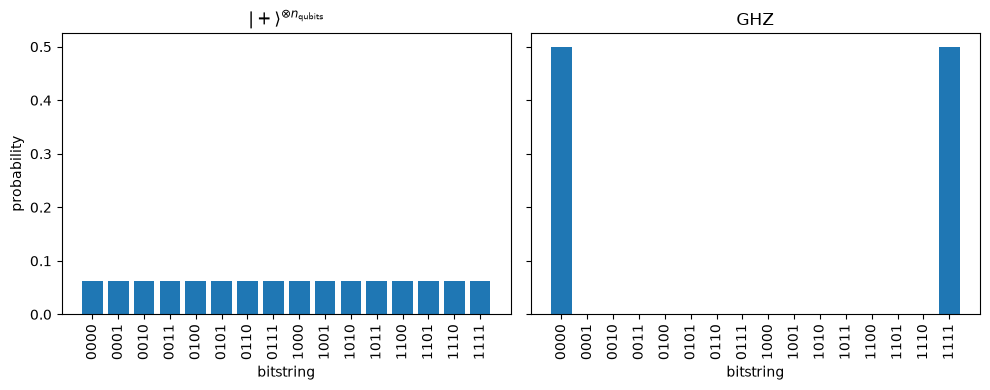

../_images/tutorials_size_dep_states_ops_10_0.png

Expectation values

Size-dependent states and operators can be combined freely to compute the expectation value of an operator on a state.

For instance, the end-to-end correlator $\langle Z_0 Z_{n-1} \rangle$ distinguishes the GHZ state (for which it is $1$ ) from $|+\rangle^{\otimes n}$ (for which it is $0$ ), while both states are eigenstates of $X^{\otimes n}$ with eigenvalue $1$ , regardless of the number of qubits:

for n in range(2, 5):
    ghz = get_state(n_qubits=n, state_class=state_class, state_name="ghz")
    plus = get_state(n_qubits=n, state_class=state_class, state_name="plus")
    zz, xx = end_to_end_zz(n), x_parity(n)
    print(
        f"n={n}: "
        f"_ghz={zz.expect(ghz).real:+.2f}, "
        f"_plus={zz.expect(plus).real:+.2f}, "
        f"_ghz={xx.expect(ghz).real:+.2f}, "
        f"_plus={xx.expect(plus).real:+.2f}"
    )

n=2: <ZZ>_ghz=+1.00, <ZZ>_plus=+0.00, <X..X>_ghz=+1.00, <X..X>_plus=+1.00
n=3: <ZZ>_ghz=+1.00, <ZZ>_plus=+0.00, <X..X>_ghz=+1.00, <X..X>_plus=+1.00
n=4: <ZZ>_ghz=+1.00, <ZZ>_plus=+0.00, <X..X>_ghz=+1.00, <X..X>_plus=+1.00

Previous
Phase Shifts and Virtual Z gates Next
Optimal Control for AFM State Preparation